Final Report

Motivation

One of our group members’ had the unfortunate experience of getting her car towed last year, due to parking near by a fire hydrant in Minnesota. It sparked our particular interest in the fire hydrant parking violations and caused us to want to investigate parking violations at large.

We are curious to know about where fire hydrant parking violations are most common in the city (perhaps to help our friend to be cautious in such areas), but we also understand that these specific violations are only a subset of all parking violations. We hope to first answer some basic questions (that may lead to other questions) about parking violations in the city and then focus in on fire hydrant parking violations specifically.

Questions and Planned Analyses

Which borough had the most violations? Which borough paid the most in fines?
What did the distribution of violations look like over other variables in the dataset borough, date, vehicle type?
Were the number of parking violations related to fire hydrants the same across the five boroughs? Can we find the hydrants that seem to be ticketed the most commonly?

Data Processing and Cleaning

We used three datasets from NYC OpenData to construct our main dataset for analysis and also utilized a few other datasets (both available online and scraped from the internet) to supplement our analysis

Open Parking and Camera Violations (dataset)

The Open Parking and Camera Violations dataset hosted online contains data on 73.6 million parking violations from 2016 to 2021. We filtered the dataset on the website page to remove redundant information and downloaded the dataset after filtering, as it was too large to download outright. We stored the dataset in a Google Drive folder, as it exceeded the size limits for GitHub.

For the process of data cleaning, we first organized all locations into the five boroughs that we are interested, Manhattan, Kings, The Bronx, State Island, and Queens. Then we changed the format of the issue_date, and separate it into month, date and year, and separated the time of the day into hour and min for further analysis. Furthermore, we found out that the data size for November and December is much smaller comparing to the other months, and we downloaded this dataset in November where the December data should not be there at that time. So we decided to only keep the data from January 1st to October 31th. Finally, we filtered out all the missing values.

After the data cleaning, here are the variables that we will be focused on:

summons_number: unique violation identifier
borough: borough violation was issued in
issue_date (also split into month, date, year): date violation was issued on
weekday: day of the week violation was issued
hour and min: time violation was issued

violation1 <-
  read_csv("data/Open_Parking_and_Camera_Violations.csv") %>% 
  janitor::clean_names() %>%
  rename(borough = county) %>%  # rename county to borough
  mutate(
    borough = case_when(
      borough %in% c("BK","K", "Kings") ~ "Brooklyn",
      borough %in% c("BX", "Bronx") ~ "Bronx",
      borough %in% c("Q", "QN", "Qns") ~ "Queens",
      borough %in% c("ST", "R", "Rich", "RICH") ~ "Staten Island",
      borough %in% c("NY", "MN") ~ "Manhattan"),
      issue_date = as.Date(issue_date, format = "%m/%d/%Y"),
      weekday = weekdays(issue_date),
      year = year(issue_date),
      month = month(issue_date),
      day = day(issue_date)
  )  %>%  # make the borough the same 
  filter(borough != "A", 
         weekday != "NA",
         month != "11",
         month != "12") %>%
  separate(violation_time, c("hour", "min"), ":") %>%
  mutate(hour = ifelse(substr(min, 3, 3) == "P", as.numeric(hour) + 12, hour)) %>%
  mutate(hour = as.numeric(hour))

Parking Violations Issued - Fiscal Year 2021 (dataset)

The Parking Violations Issued - Fiscal Year 2021 dataset provides information about the violations issued during the respective fiscal year. This dataset provides us with approximate locations where each parking violation was issued. In addition, this dataset also provides us with information about the car type.

We then combined this dataset with the first dataset by the summons_number. These are the variables that we are interested in for further analysis:

summons_number: unique violation identifier, used to join dataset with the Open Parking dataset
geo_nyc_address: combination of a few address components in the raw data, passed into NYCGeoSearch in mapping analysis
vehicle_body_type: type of vehicle the violation was issued to
vehicle_year: year of the vehicle

violation2 <- 
  read_csv("data/Parking_Violations_Issued_-_Fiscal_Year_2022.csv") %>%
  janitor::clean_names() %>%
  rename(borough = violation_county) %>%
  select(house_number,
         street_name,
         intersecting_street,
         summons_number, 
         vehicle_body_type, 
         vehicle_year)
violation <-
  violation1 %>% left_join(violation2, by = "summons_number") %>%
  mutate(
    house_street = ifelse(is.na(street_name), NA, ifelse(is.na(house_number), paste("0", street_name), paste(house_number, street_name))),
    geo_nyc_address = paste(house_street[!is.na(house_street)], 
                            intersecting_street[!is.na(intersecting_street)], 
                            paste(toupper(borough), "COUNTY"),
                            "NEW YORK, NY",
                            sep = ","),
    google_address = paste(house_street[!is.na(house_street)], 
                           intersecting_street[!is.na(intersecting_street)], 
                           toupper(borough), 
                           "New York, NY",
                           sep = ",")
  ) %>%
  select(-house_number, -street_name, -intersecting_street)

 address_std <- function(ad){
  address <- 
    toupper(ad) %>%
    str_replace(" PKY,", " PARKWAY, ") %>%
    str_replace(" BLVD,", " BOULEVARD, ") %>%
    str_replace(" BL,", "BOULEVARD, ") %>%
    str_replace(" AVE,", " AVENUE, ") %>%
    str_replace(" AV,", "AVENUE, ") %>%
    str_replace(" ST,", " STREET, ") %>%
    str_replace(" PL,", " PLACE, ") %>%
    str_replace(" HWY,", "HIGHWAY, ") %>%
    str_replace(" DR,", "DRIVE, ")
  return(address)
}

violation <- violation  %>% mutate(geo_nyc_address = geo_nyc_address %>% address_std())

Hydrants in NYC (dataset)

This dataset contains the locations of all fire hydrants in NYC. After tidying the dataset and recoding some columns, we are most interested in the following variables:

borough: borough the hydrant is located in
unitid: unique hydrant identifier
lat and long: latitude and longitude coordinates of the hydrant

NYC COVID-19 Case Counts (dataset)

This dataset contains non-cumulative daily counts of COVID-19 cases across the five boroughs in NYC. After importing and tidying the dataset, we are interested in the following variables:

borough: borough of interest/measurement
new_Cases: count of daily new COVID_19 cases
date_of_interest: the date the case count is associated with

EDA

In order to have a better understanding of the datasets and trends of parking violations in the city may follow, we conducted some exploration mainly through visualization.

We first tried to explore the overall distribution of the parking violation frequency. Then, we tried to investigate how the number of parking violations distributed over month, week, time of the day and vehicle type. Finally, we looked at the distribution of fine amounts by boroughs.

Violation Frequency

We first want to get a feel for the distribution of violations across the five boroughs. We will construct a bar chart tabulating the number of parking violations incurred in each of the five boroughs.

Distribution of Parking Violation

violation1 %>% 
  count(borough) %>% 
  mutate(
    borough = fct_reorder(borough, n)
    ) %>% 
  ggplot(aes(x = borough, y = n, fill = borough)) + 
  geom_bar(stat = "identity") + 
  labs(
    title = "Frequency of Tickets by Borough",
    x = "Borough",
    y = "Number of Tickets",
    fill = "Borough") +
  theme(
    axis.text.x = element_blank()
  )

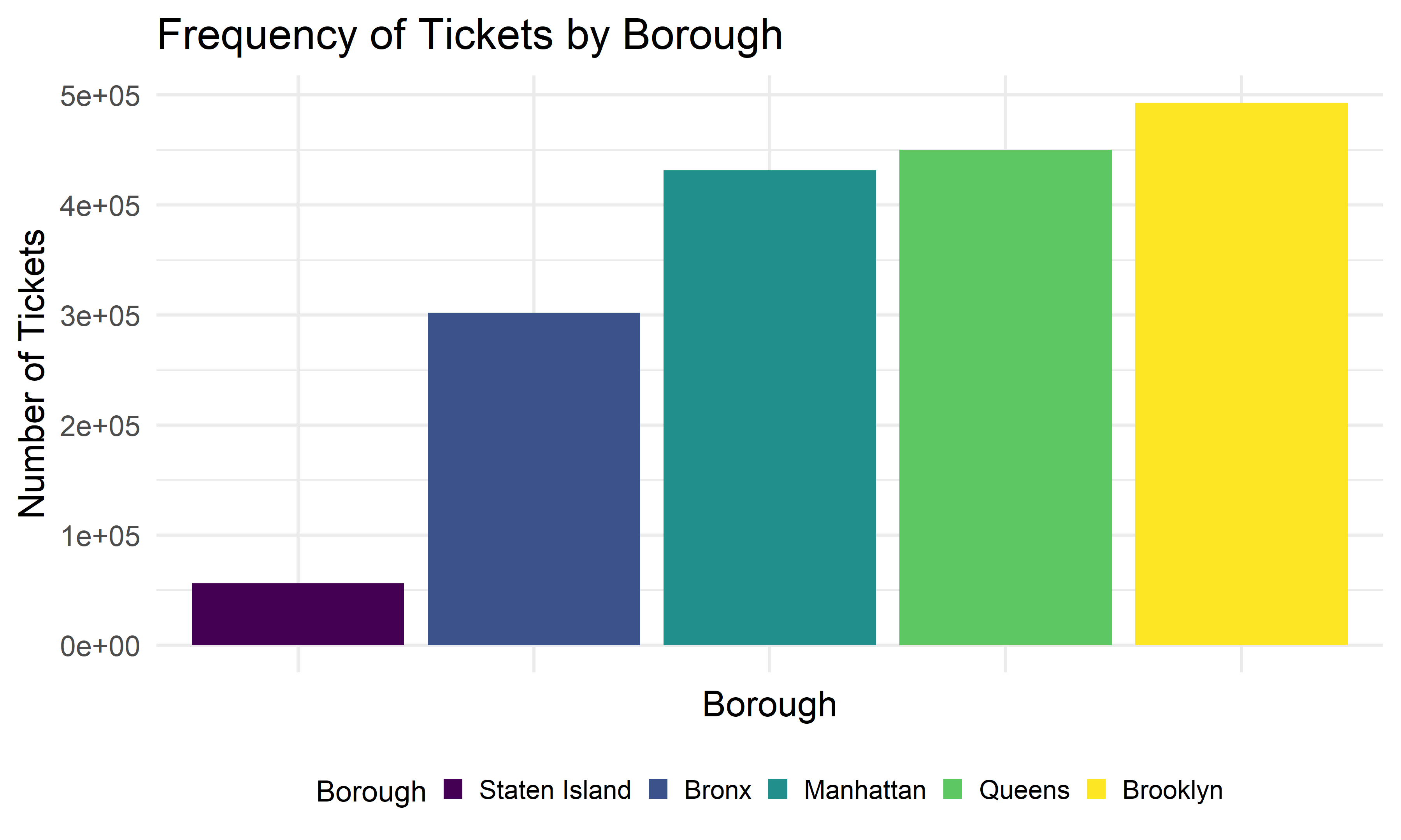
Brooklyn has the greatest number of tickets among five boroughs. Staten Island has the lowest number of tickets in 2021.

The bar graph further break down the number of tickets in five borough from January to October in 2021. There is sharp increasing of number of tickets in October. The distribution of number of tickets are similar from January to October across Borough. Brooklyn has the highest number of tickets, while State Island has the least number of tickets. There is large increase in number of tickets in October in all boroughs except Staten Island.

violation1 %>% 
  group_by(borough) %>%
  count(month) %>% 
  mutate(month = month.abb[as.numeric(month)],
         month = fct_relevel(month, c("Jan", "Feb", "Mar", "Apr","May","Jun", "Jul", "Aug", "Sep", "Oct"))) %>% 
  ggplot(aes(x = month, y = n, fill = borough)) +
  geom_bar(stat = "identity",
           position = "dodge") +
  labs(
    title = "Frequency of Tickets in Boroughs",
    x = "Month",
    y = "Number of Tickets in Each Month",
    fill = "Borough")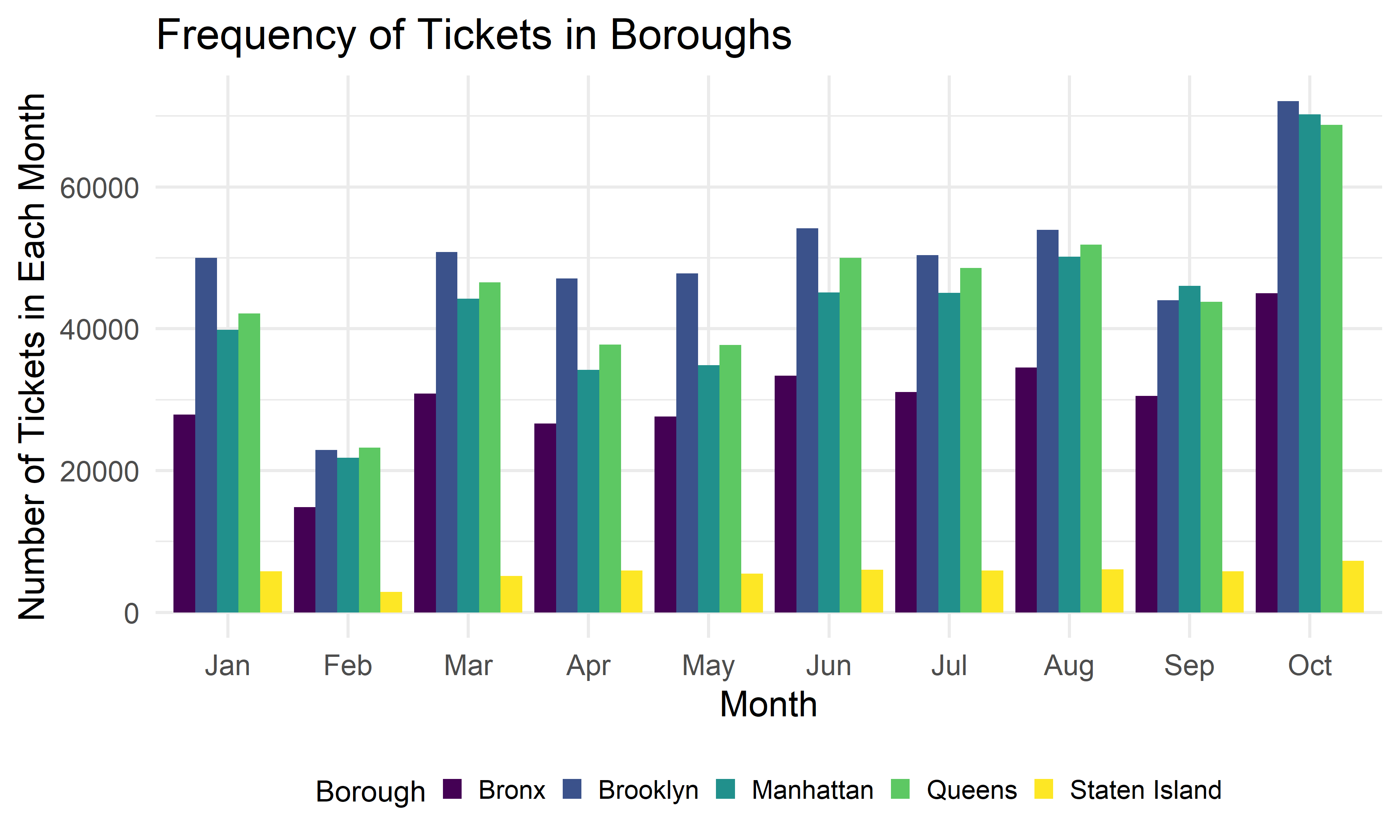

Top 10 Violations in NYC in 2021

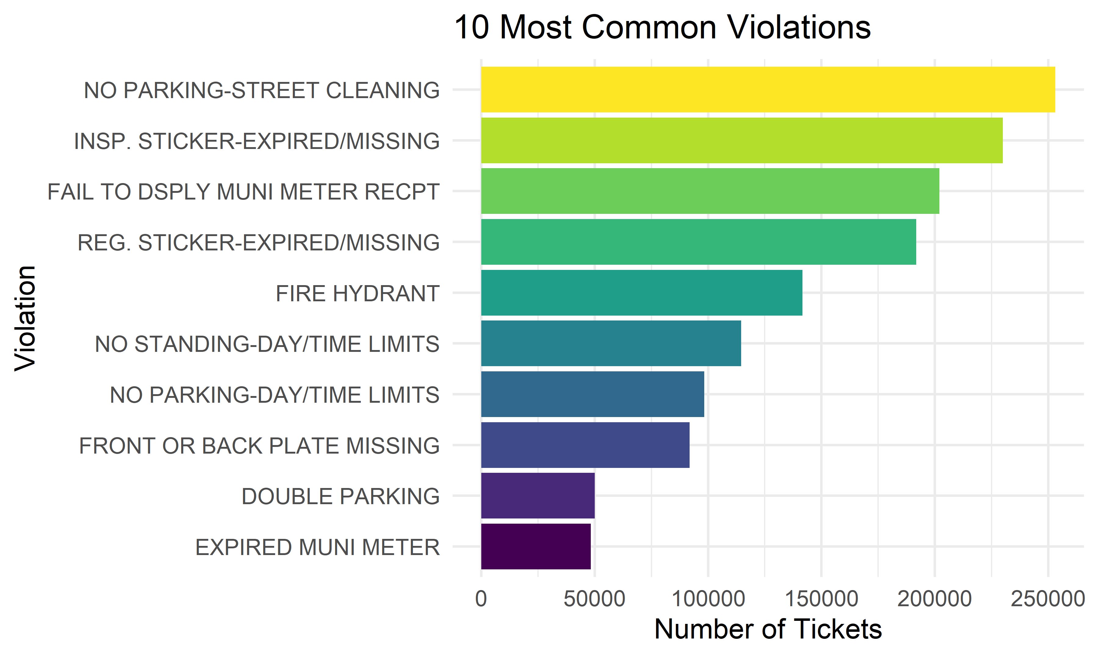
We want to know the most common ten violation types based on the total frequency in NYC in 2021.

total_violation = violation1 %>% 
  count(violation) %>% 
  mutate(
    violation = fct_reorder(violation, n),
    ranking = min_rank(desc(n))
  ) %>% 
  filter(ranking <= 10) %>% 
  arrange(n)

total_violation %>% 
  ggplot(aes(x = violation, y = n, fill = violation)) + 
  geom_bar(stat = "identity") +
  labs(title = "10 Most Common Violations",
       x = "Violation",
       y = "Number of Tickets",
       fill = "Violation") + coord_flip() +
  theme(legend.position = "none"
        )

Top 5 Violation Types Across Boroughs

We want to find the top five common violation types in each borough, and see whether there exists difference among boroughs. We found that the most common 5 reasons of getting a violation tickets in NYC among all five boroughs are: 1) No parking-street cleaning, 2) Failure to display a muni-meter receipt, 3) Inspection sticker-expired/missing, 4) Registration sticker-expired /missing, and 5) Fire hydrant.

## top 5 reasons of violation tickets
violation_type = violation1 %>% 
  group_by(borough) %>% 
  count(violation) %>% 
  mutate(
    violation = fct_reorder(violation, n),
    index = min_rank(desc(n))) %>% 
  filter(index <= 5)  %>%
  arrange(index)

Bronx

bronx_vio_type = 
  violation_type %>% 
  filter(borough == "Bronx") %>% 
  ggplot(aes(x = index, y = n, fill = violation)) + 
  geom_bar(stat = "identity") + 
  labs(
    title = "Top 5 Parking Violation Types in Bronx (2021)", 
    x = "Violation Type", 
    y = "Number of tickets") +
  theme(
    axis.text.x = element_blank(),
    legend.text = element_text(size = 8),
    legend.key.size = unit(.5,"line"),
    legend.position = "right")
bronx_vio_type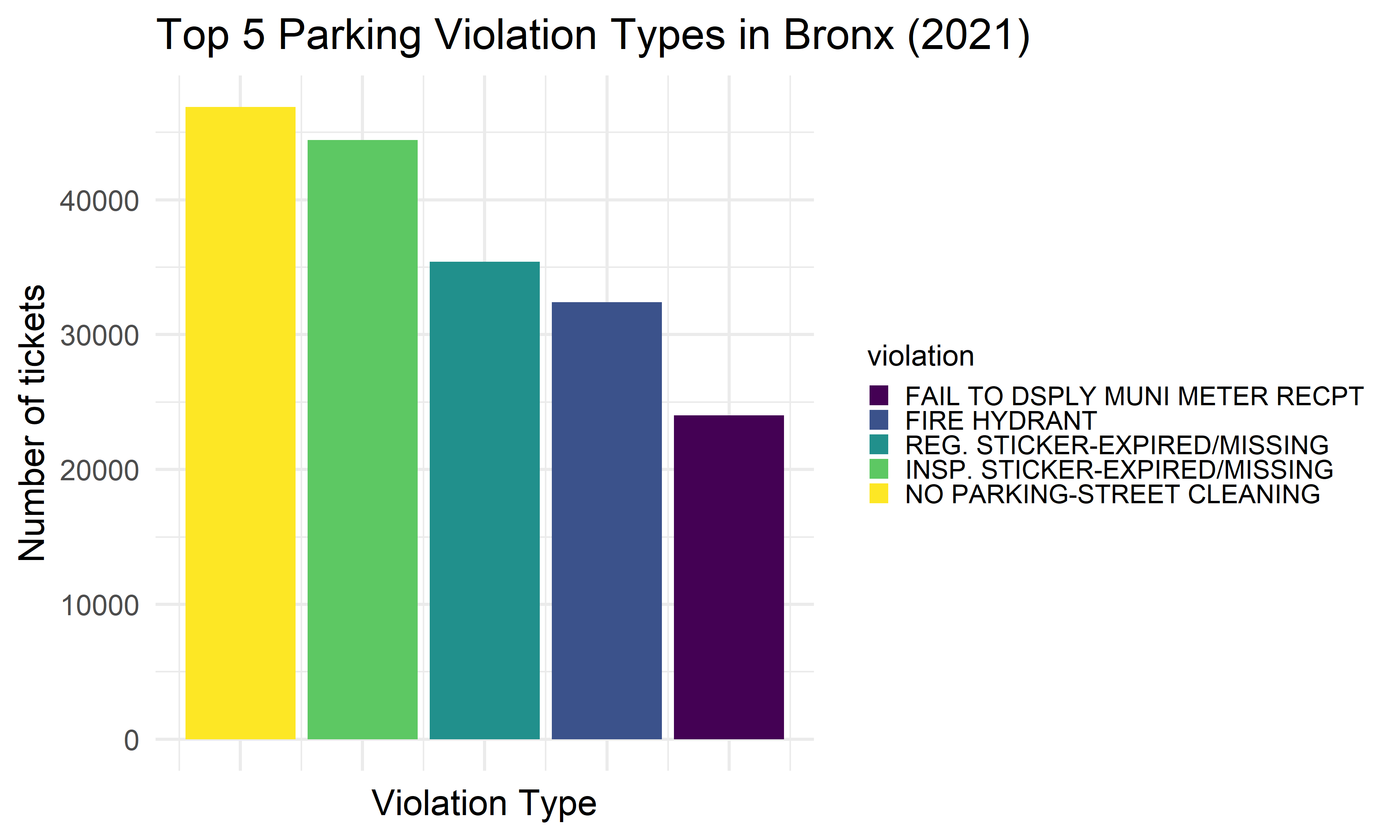

Brooklyn

brooklyn_vio_type = 
  violation_type %>% 
  filter(borough == "Brooklyn") %>% 
  ggplot(aes(x = index, y = n, fill = violation)) + 
  geom_bar(stat = "identity") + 
  labs(
    title = "Top 5 Parking Violation Types in Brooklyn (2021)", 
    x = "Violation Type", 
    y = "Number of tickets") +
  theme(
    axis.text.x = element_blank(),
    legend.text = element_text(size = 8),
    legend.key.size = unit(.5,"line"),
    legend.position = "right")

brooklyn_vio_type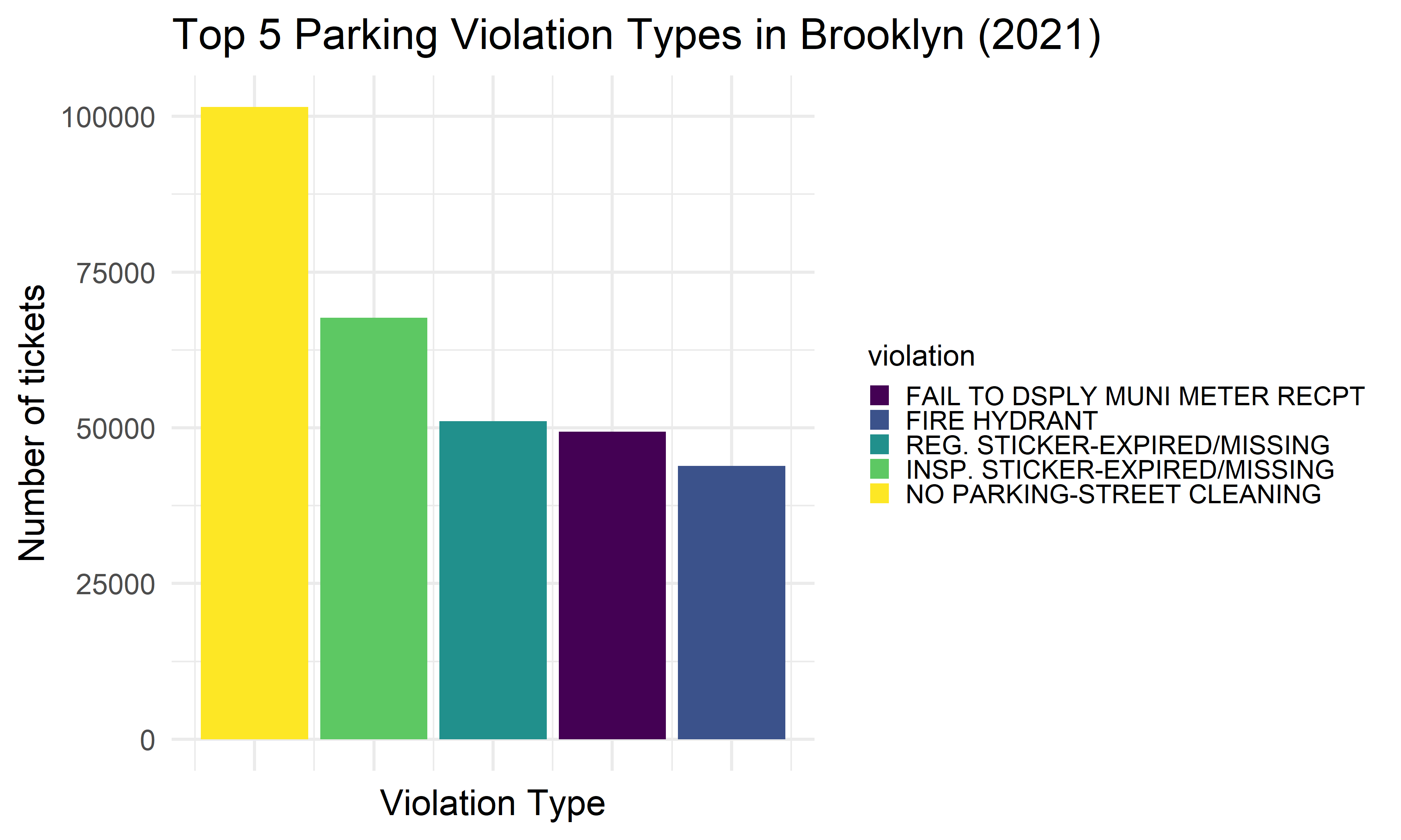

Manhattan

manhattan_vio_type = 
  violation_type %>% 
  filter(borough == "Manhattan") %>% 
  ggplot(aes(x = index, y = n, fill = violation)) + 
  geom_bar(stat = "identity") + 
  labs(
    title = "Top 5 Parking Violation Types in Manhattan (2021)", 
    x = "Violation Type", 
    y = "Number of tickets") +
 theme(
    axis.text.x = element_blank(),
    legend.text = element_text(size = 8),
    legend.key.size = unit(.5,"line"),
    legend.position = "right")

manhattan_vio_type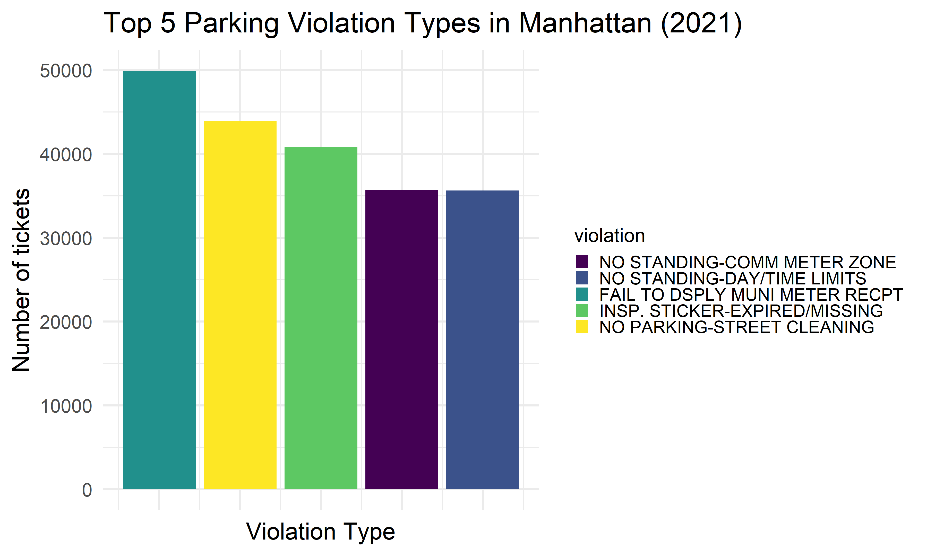

Queens

queens_vio_type = 
  violation_type %>% 
  filter(borough == "Queens") %>% 
  ggplot(aes(x = index, y = n, fill = violation)) + 
  geom_bar(stat = "identity") + 
  labs(
    title = "Top 5 Parking Violation Types in Queens (2021)", 
    x = "Violation Type", 
    y = "Number of tickets") +
  theme(
    axis.text.x = element_blank(),
    legend.text = element_text(size = 8),
    legend.key.size = unit(.5,"line"),
    legend.position = "right")

queens_vio_type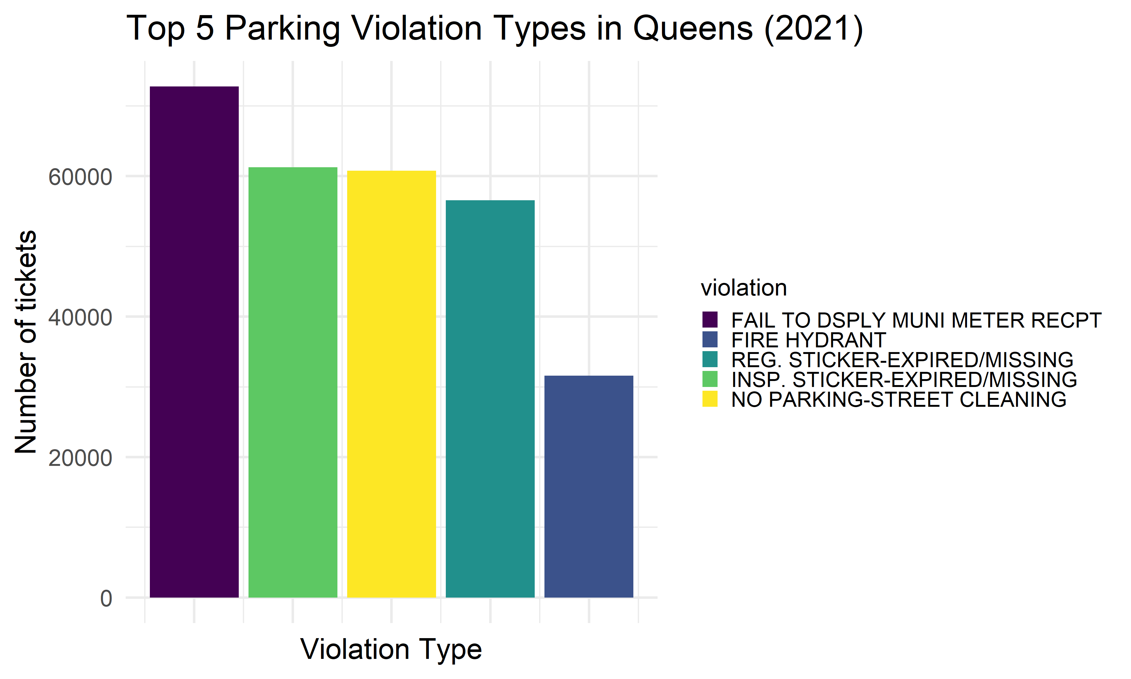

Staten Island

si_vio_type = 
  violation_type %>% 
  filter(borough == "Staten Island") %>% 
  ggplot(aes(x = index, y = n, fill = violation)) + 
  geom_bar(stat = "identity") + 
  labs(
    title = "Top 5 Parking Violation Types in Staten Island (2021)", 
    x = "Violation Type", 
    y = "Number of tickets") +
  theme(
    axis.text.x = element_blank(),
    legend.text = element_text(size = 8),
    legend.key.size = unit(.5,"line"),
    legend.position = "right")

si_vio_type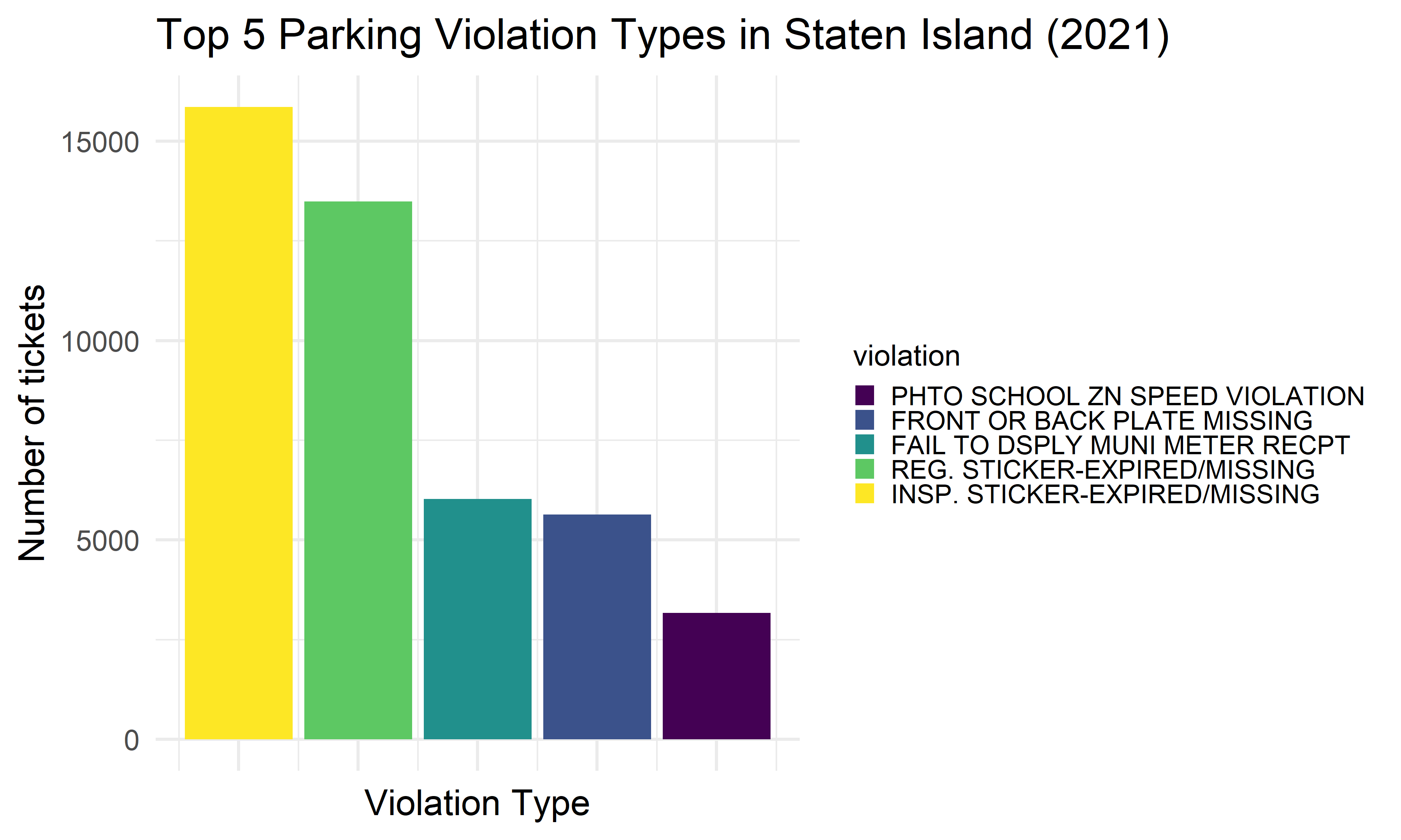

Violations by Vehicle Body Type

The following plot describes the frequency of violation by vehicle body types. There are mainly top 5 types of vehicle body at the top 5 ranking(unknown type excluded), which are SDN, PICK, 2DSD, 4DSD, SUBN. The type abbreviations are the exact match of the body type listed on the vehicle registration. The law defines a suburban(SUBN) as a vehicle that can be used to carry passengers and cargo. Other common body types and codes for vehicles registered in the passenger vehicle class are sedan (SDN), a two-door sedan (2DSD) and a four-door sedan (4DSD), pick-up trucks (PICK).

gg_vio_bt = 
  violation %>%
  count(vehicle_body_type) %>% 
  mutate(
    vehicle_body_type = fct_reorder(vehicle_body_type, n) 
  ) %>% 
  filter(
    vehicle_body_type != "NA",
    n > 10000
  ) %>% 
  ggplot(aes(x = vehicle_body_type, y = n, fill = vehicle_body_type)) +
  geom_bar(stat = "identity") +
  labs(
    title = "Frequency of Violation by Vehicle Body Type",
    x = "Vehicle Body Types",
    y = "Count", 
    fill = "Vehicle Body Type"
  ) +
  geom_text(aes(label = n), position = position_dodge(width = 0.9), vjust = -0.25)

gg_vio_bt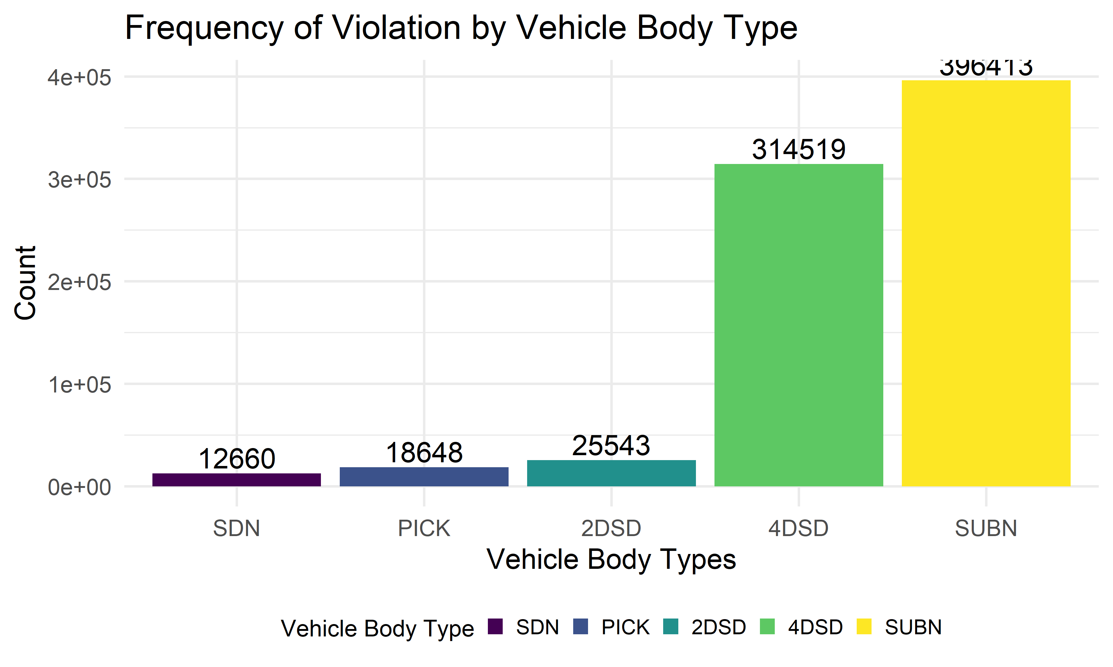

Violation by Vehicle Type

Fine Amount

Payment Amount by Borough

payment_by_borough <- violation %>% filter(payment_amount != 0)
fig1 <- plot_ly(payment_by_borough, x = ~payment_amount, color = ~borough, type = "box", colors = "viridis")
fig1 %>% layout(yaxis = list(showticklabels = FALSE),
               title = "<b>Payment by Borough</b>",
                xaxis = list(title = "Payment Amount"))

We see that the median payment amount is approximately the same across the five boroughs, around $60-65. However, it seems that the payment amount distributions in the Bronx, Brooklyn, and Manhattan all have a significant right skew. This likely just indicates that the distribution of violation types differ across the five boroughs.

Payment Amount by Violation

payment_by_violation <- violation %>% filter(payment_amount != 0)
fig2 <- plot_ly(payment_by_violation, x = ~payment_amount, color = ~violation, type = "box", colors = "viridis")
fig2 %>% layout(yaxis = list(showticklabels = FALSE),
                title = "<b>Payment Amount by Violation Type</b>",
                xaxis = list(title = "Payment Amount"))

We see that the distribution of payment amounts can vary significantly between violation types.

Fire Hydrant Violation Payment Amount by Borough

fire_hydrant_violation_payment <- violation %>% filter(payment_amount != 0, violation == "FIRE HYDRANT")
fig3 <- plot_ly(fire_hydrant_violation_payment, x = ~payment_amount, color = ~borough, type = "box", colors = "viridis")
fig3 %>% layout(yaxis = list(showticklabels = FALSE),
                title = "<b>Fire Hydrant Payment Amount by Borough</b>",
                xaxis = list(title = "Payment Amount"))

Finally, we see here that the distribution of fire hydrant payment amounts is about the same across the five boroughs. It appears that most recipients of this violation will pay at most $115.

Fine Amount

Violation over Time

Now, we want to use visualization over time to find out some pattern of parking violation frequency in NY in 2021. We want to know how month, weekday and specific time of the day are associated with the parking violation counts.

Monthly Ticket Totals by Borough

knitr::opts_chunk$set(
  fig.width = 6,
  fig.asp = .6,
  out.width = "90%"
)

violation %>%
  mutate(month = month.name[as.numeric(month)]) %>%
  mutate(month = as.factor(month),
         month = fct_relevel(month, "January", "February", "March", "April", "May", "June", "July", "August", "September", "October")) %>%
  relocate(month) %>%
  group_by(borough, month) %>%
  summarize(n_obs = n()) %>%
  ggplot(aes(x = month, y = n_obs, group = 1, color = borough)) + 
  geom_point() + geom_line() + 
  theme(axis.text.x = element_text(angle = 60, hjust = 1, size = 5) ) +
  labs(
    title = "Total Parking Violations by Month and Borough",
    x = "Month",
    y = "Total Violations"
    ) +
  facet_wrap(~ borough, nrow = 1)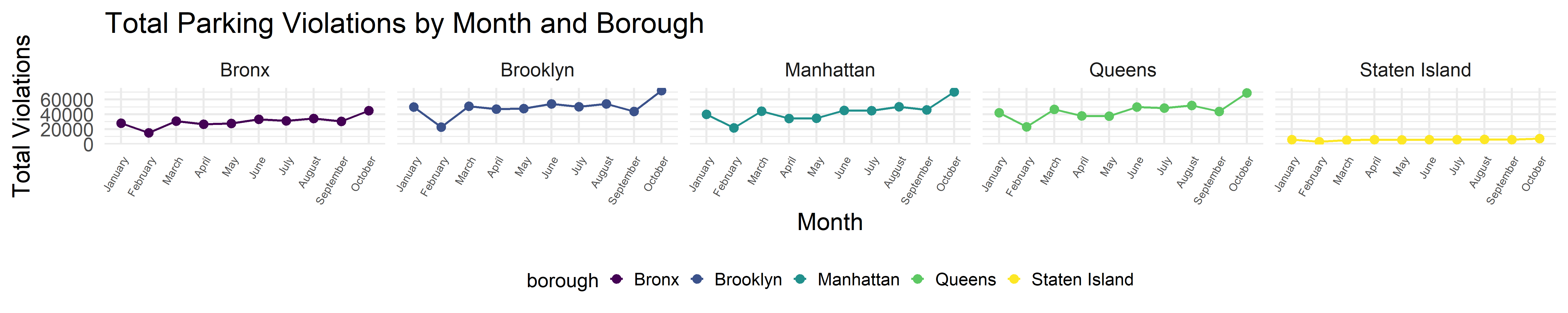

The above plot shows the total number of parking violation within each month for different boroughs. From the plot we can see that all boroughs have a similar pattern, the total violation counts in February is lower, and the total violation counts in October is higher comparing to other months. We can also see that total violation count in Staten Island is much more lower than the other four boroughs.

Ticket Time Series by Borough

violation %>%
  group_by(borough, issue_date) %>%
  summarize(n_obs = n()) %>%
  ggplot(aes(x = issue_date, y = n_obs, color = borough)) + 
  geom_line() + 
  labs(title = "Total Parking Violations Time Series by Borough",
       x = "Issue Date",
       y = "Total Violations",
       color = "Borough") +
  facet_wrap(~ borough, nrow = 5, scales = "free_y")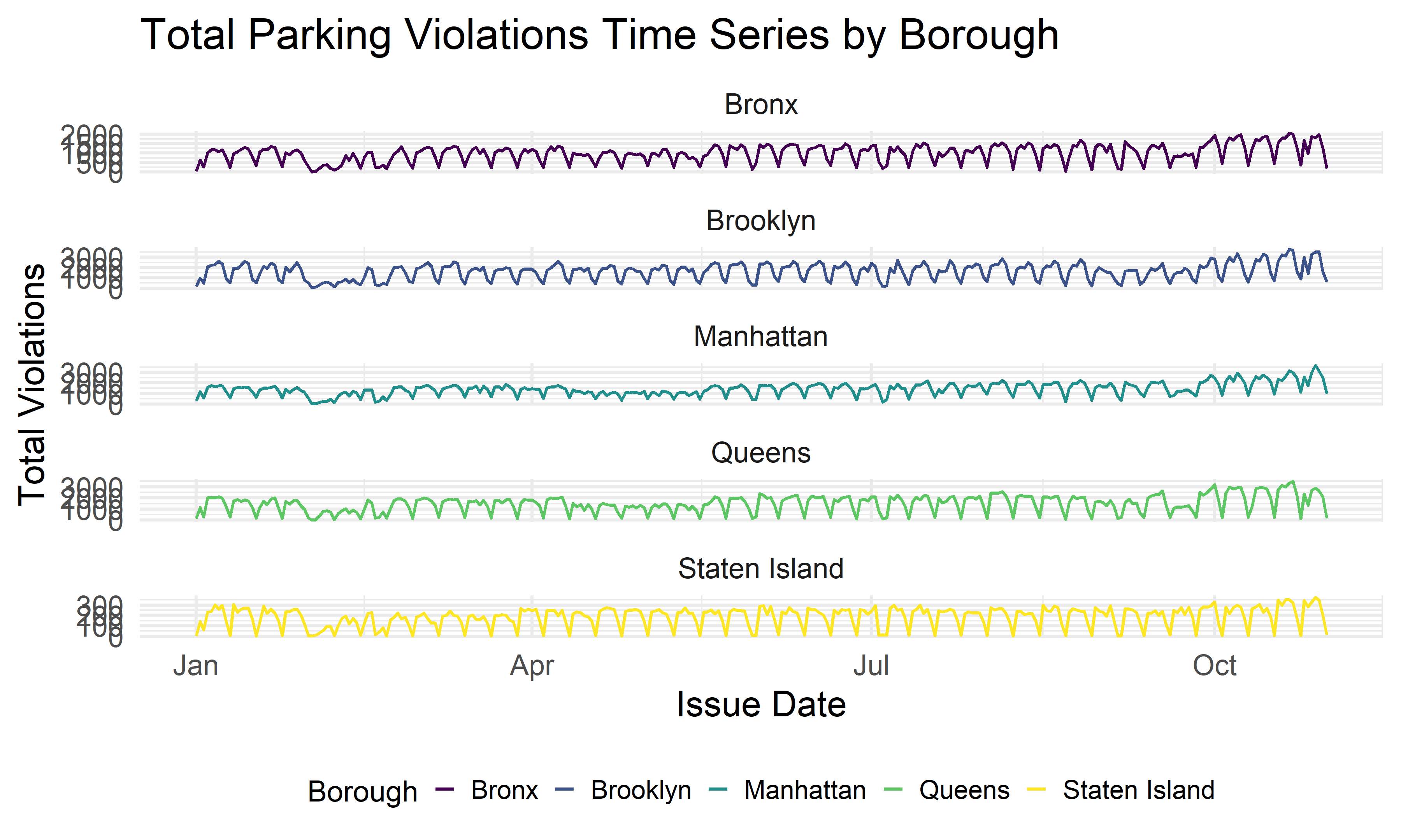

After visualizing the monthly pattern, we also want to know if there is any pattern within each month. The above plot shows the total daily parking violation counts for each month by borough. We see there is a pattern in the fluctuation of total tickets day by day.

Cumulative Weekday Ticket Analysis by Borough

violation %>% 
  mutate(weekday = as.factor(weekday)) %>%
  mutate(weekday = fct_relevel(weekday, "Monday", "Tuesday", "Wednesday", "Thursday", "Friday", "Saturday", "Sunday")) %>%
  relocate(weekday) %>%
  group_by(borough, weekday) %>%
  summarize(n_obs = n()) %>%
  ggplot(aes(x = weekday, y = n_obs, group = 1, color = borough)) + 
  geom_point() + geom_line() + 
  theme(axis.text.x = element_text(angle = 60, hjust = 1) ) + 
  facet_wrap(~ borough, nrow = 1) +
  labs(
    title = "Total Parking Violations by Weekday and Borough",
    x = "Weekday",
    y = "Total Violations",
    color = "Borough"
    )

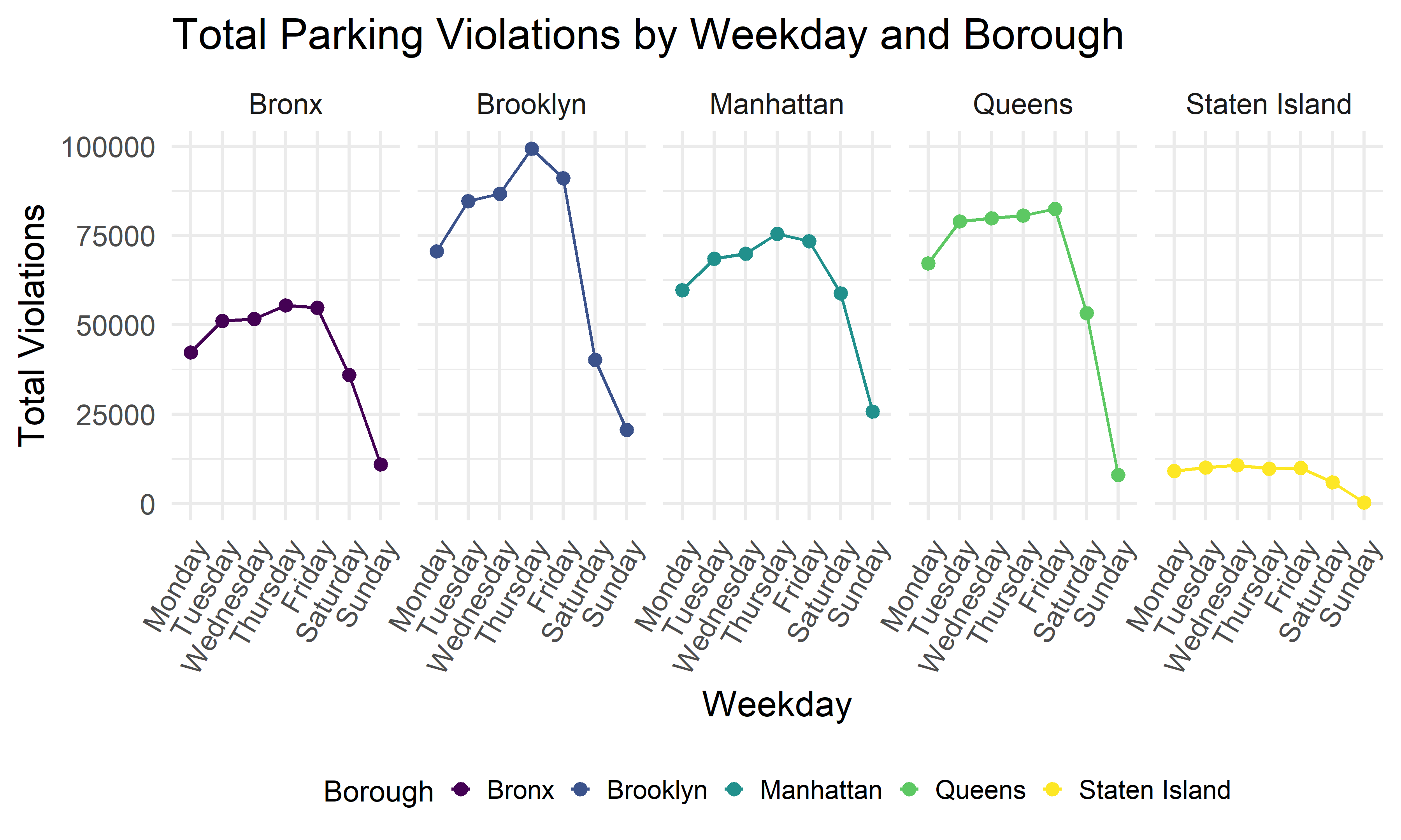
In order to explore more of the weekly parking violation pattern, we plot the violation counts of each weekday for every borough. We can see that all boroughs have a similar pattern, where Saturday has the lowest violation counts and Friday had the second lowest counts comparing to all other weekdays.

Cumulative Hourly Ticket Analysis by Borough

violation %>%
  mutate(hour = as.numeric(hour)) %>%
  group_by(borough, hour) %>%
  summarize(n_obs = n()) %>%
  filter(hour <= 24) %>%
  ggplot(aes(x = hour, y = n_obs, color = borough)) + geom_point() + geom_line() +
  labs(title = "The total number of violations during 24 hours \n of a day in 2021 for each borough") +
  facet_wrap(~ borough, nrow = 2)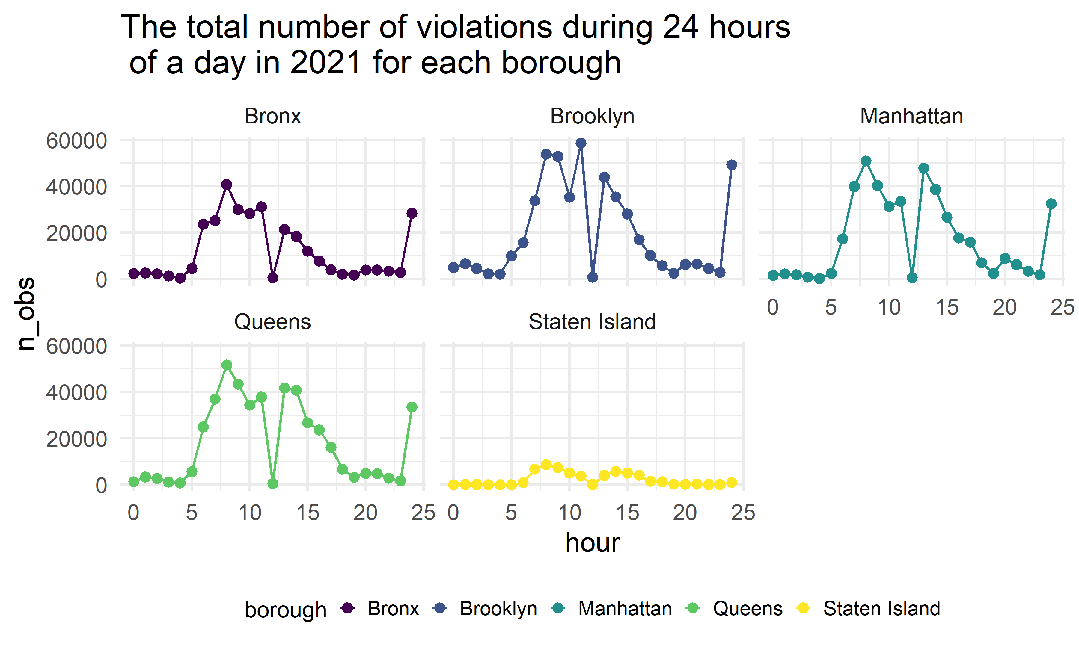

Furthermore, we also try to explore the 24-hour violation pattern within a day. From the above plot, all boroughs also show a similar daily pattern. The number of violations tends to increase from 6:00 AM to 8:00 AM, remain high in 8:00 AM to 2:00 PM, decrease from 2:00PM to 7:00 PM, and remain low from 7:00 PM to 5:00 AM.

Violation Timeline

Fire Hydrants Violation

hydrant <- 
  violation %>% 
  filter(violation %in% c("FIRE HYDRANT"), !is.na(geo_nyc_address))

As one of our group members has suffered personal loss as a result of parking near a fire hydrant, we want to do more exploration on fire hydrant violations. We want to see how the number of fire hydrant violations are distributed across each borough and over time in NYC (to help her avoid being a part of such statistics).

Hydrant Violations by Borough

hydrant %>%
  group_by(borough) %>%
  summarise(n_obs = n()) %>%
  mutate(
    borough = fct_reorder(borough, n_obs) 
  ) %>% 
  ggplot(aes(x = borough, y = n_obs, fill = borough)) + geom_bar(stat = "identity") +
  labs(
    title = "Frequency of Fire Hydrant Violations by Borough",
    x = "Borough",
    y = "Number of Violations"  ) +
  geom_text(aes(label = n_obs), position = position_dodge(width=0.9), vjust = -0.25) +
  theme(legend.position = "none")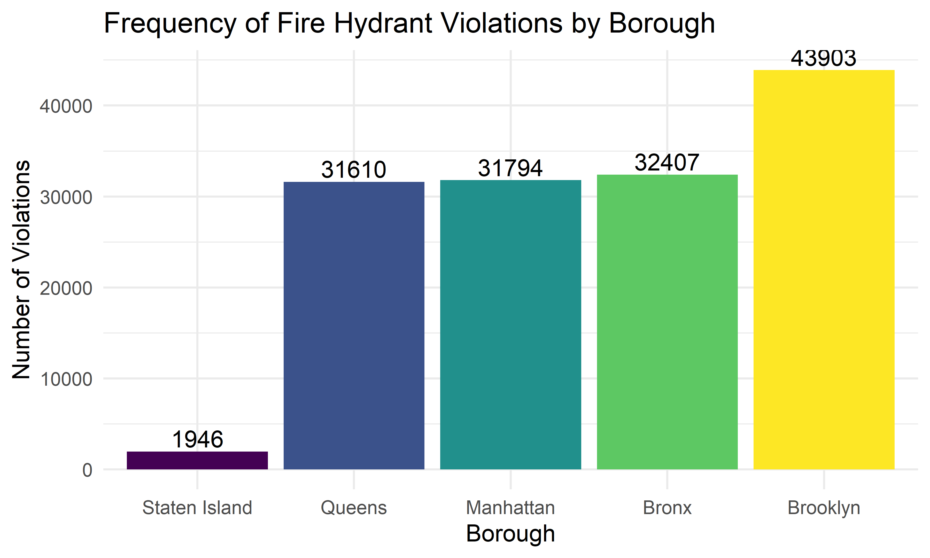

From the above bar charts, we can see that Staten Island has the fewest number of fire hydrant violations and Brooklyn has the highest number of fire hydrant violations, which is consistent with the total violations across boroughs we found before.

Hydrant Violations by Month

hydrant %>%
  mutate(month = month.name[as.numeric(month)]) %>%
  mutate(month = as.factor(month),
         month = fct_relevel(month, "January", "February", "March", "April", "May", "June", "July", "August", "September", "October")) %>%
  relocate(month) %>%
  group_by(borough, month) %>%
  summarize(n_obs = n()) %>%
  ggplot(aes(x = month, y = n_obs, group = 1, color = borough)) + 
  geom_point() + geom_line() + 
  theme(axis.text.x = element_text(angle = 60, hjust = 1, size = 5) ) +
  labs(title = "Fire Hydrant Violations by Month and Borough",
       color = "Borough",
       y = "Number of Violations",
       x = "Month"
       ) + facet_wrap(~ borough, nrow = 1)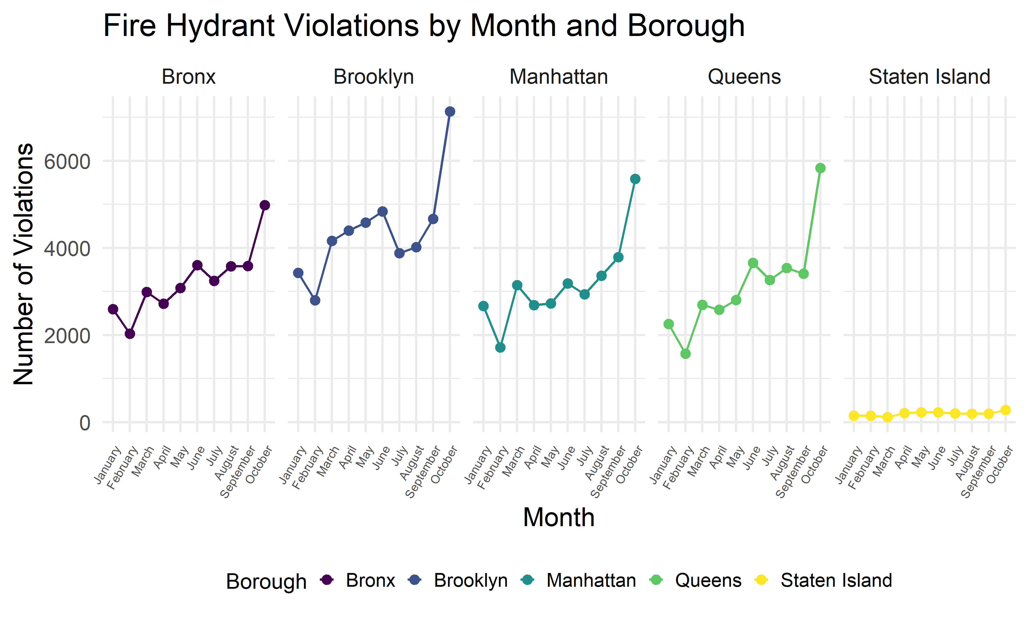

This plot shows the number of fire hydrant violations within each month for different boroughs. We can see that all boroughs have a similar pattern, the total violation counts in February is lower, and the total violation counts in October is higher comparing to other months. It’s also quite consistent with the pattern we found for the total number of violations above.

Fire Hydrant Violations

Statistical Analysis

Does the total daily number of parking violations issued vary over the year?

We have seen that it seems that time is associated with the parking violations that are issued, as it seems that the number of violations issued varies over the course of the year. We performed a one-way ANOVA test across the weekdays and months parking violations occurred in to see whether there is significant differences within the groups of time.

ANOVA Test - Month and Violations

As from the data visualization, we observed patterns for the parking violation number over the year. In order to discuss further about how the total number of parking violations vary over the year, we will conduct a one-way ANOVA test to see if the average number of parking violations varies significantly over the months represented in this dataset.

$H_0$: The mean number of parking violation are not different across months

$H_1$: The mean number of parking violation are different across months

fit_df = violation %>%
  mutate(month = as.factor(month)) %>%
  group_by(month, weekday, day) %>%
  summarize(n_obs = n())

fit_model_month = lm(n_obs ~ month, data = fit_df)
anova(fit_model_month) %>% knitr::kable(caption = "One way ANOVA of violation frequency and month")

One way ANOVA of violation frequency and month
	Df	Sum Sq	Mean Sq	F value	Pr(>F)
month	9	494640293	54960033	9.662275	0
Residuals	294	1672302865	5688105	NA	NA

The p-value is very small in the above test. Thus, we reject the null hypothesis that the mean number of parking violations are constant across the months. There is evidence that indicates that the average number of parking violations varies across months.

COVID-19’s Association with Parking Violations

We recognize that results produced by the ANOVA test confounded by the COVID-19 pandemic, as the pandemic has certainly has caused disruptions in many spheres of everyday life. We will investigate whether the daily number of COVID-19 cases over the past year is associated with the number of parking violations.

knitr::opts_chunk$set(
  fig.width = 6,
  fig.asp = .6,
  out.width = "90%"
)

url <- "https://raw.githubusercontent.com/nychealth/coronavirus-data/master/trends/data-by-day.csv"

covid <- 
  read_csv(url(url)) %>%
  janitor::clean_names() %>%
  select(date_of_interest, bx_case_count, mn_case_count, si_case_count, qn_case_count, bk_case_count) %>%
  pivot_longer(
    cols = bx_case_count:bk_case_count,
    names_to = "borough",
    values_to = "new_cases"
  ) %>%
  mutate(
    borough_abbr = str_replace(borough, "_case_count", ""),
    borough = 
      case_when(
      borough_abbr == "bx" ~ "Bronx",
      borough_abbr == "bk" ~ "Brooklyn",
      borough_abbr == "mn" ~ "Manhattan",
      borough_abbr == "qn" ~ "Queens",
      borough_abbr == "si" ~ "Staten Island"
    ),
    date_of_interest = as.Date(date_of_interest, "%m/%d/%Y")
  ) 

violation_covid <-
  violation %>% 
  count(issue_date, borough) %>%
  rename(total_violations = n) %>%
  left_join(covid, by = c("issue_date" = "date_of_interest", "borough"))  %>%
  filter(!is.na(new_cases))

First, we will construct a scatter plot of new COVID-19 cases against total violations, colored by borough:

violation_covid %>%
  ggplot(aes(x = new_cases, y = total_violations)) +
  geom_point(alpha = 0.15, aes(col = borough)) +
  geom_smooth(se = FALSE, col = "red") +
  labs(
    x = "New COVID-19 Cases",
    y = "Total Violations",
    col = "Borough",
    title = "Total Violations vs. New COVID-19 Cases (2021)",
    caption = "Note: each point represents a single day of observation"
  )

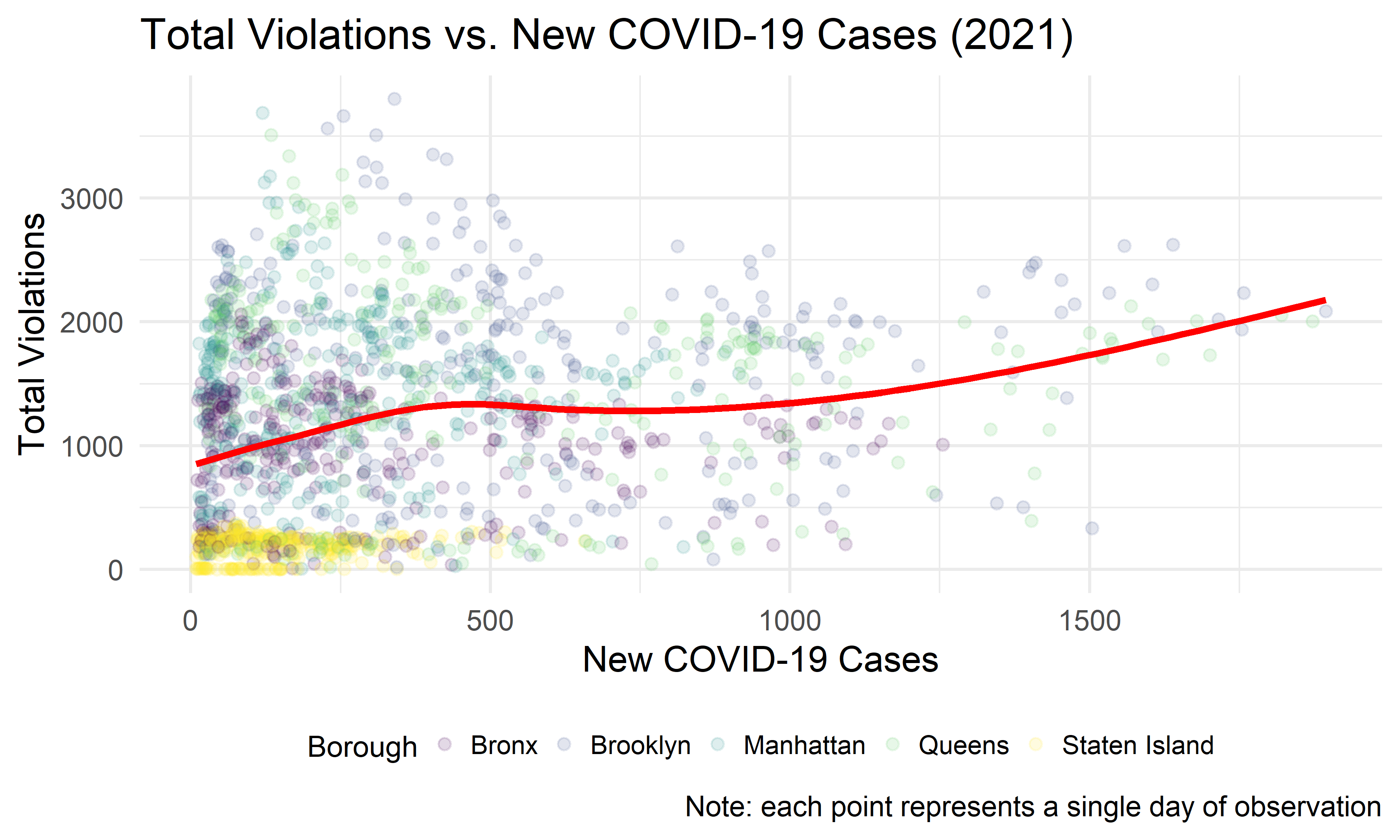
It appears that the greatest range in number of violations given out occurs when there are fewer than about 300 COVID-19 cases a day.

violation_covid_long <-
  violation_covid %>% 
  pivot_longer(
    cols = total_violations:new_cases,
    names_to = "parameter",
    values_to = "value"
  ) %>%
  mutate(
    parameter = if_else(parameter == "total_violations", "Total Violations", if_else(parameter == "new_cases", "Total New COVID-19 Cases", ""))
  )

gg_violation_covid <- 
  violation_covid_long %>% 
  ggplot(aes(x = issue_date, y = value, col = parameter)) +
  geom_line(alpha = 0.2) + 
  geom_smooth(se = FALSE) +
  xlim(c(as.Date("01-01-2021", "%m/%d/%Y"), as.Date("11-21-2021", "%m/%d/%Y"))) +
  theme(axis.text.x = element_text(angle = 90, vjust = 0.5, hjust = 1)) +
  labs(
    x = "Date",
    y  = "Count",
    col = "Parameter"
  )

(gg_violation_covid + 
    labs(title = "Total Parking Violations and New COVID-19 Cases Over Time\n(2021)") +
    theme(legend.position = "none")) / 
(gg_violation_covid  
   + facet_grid(. ~ borough))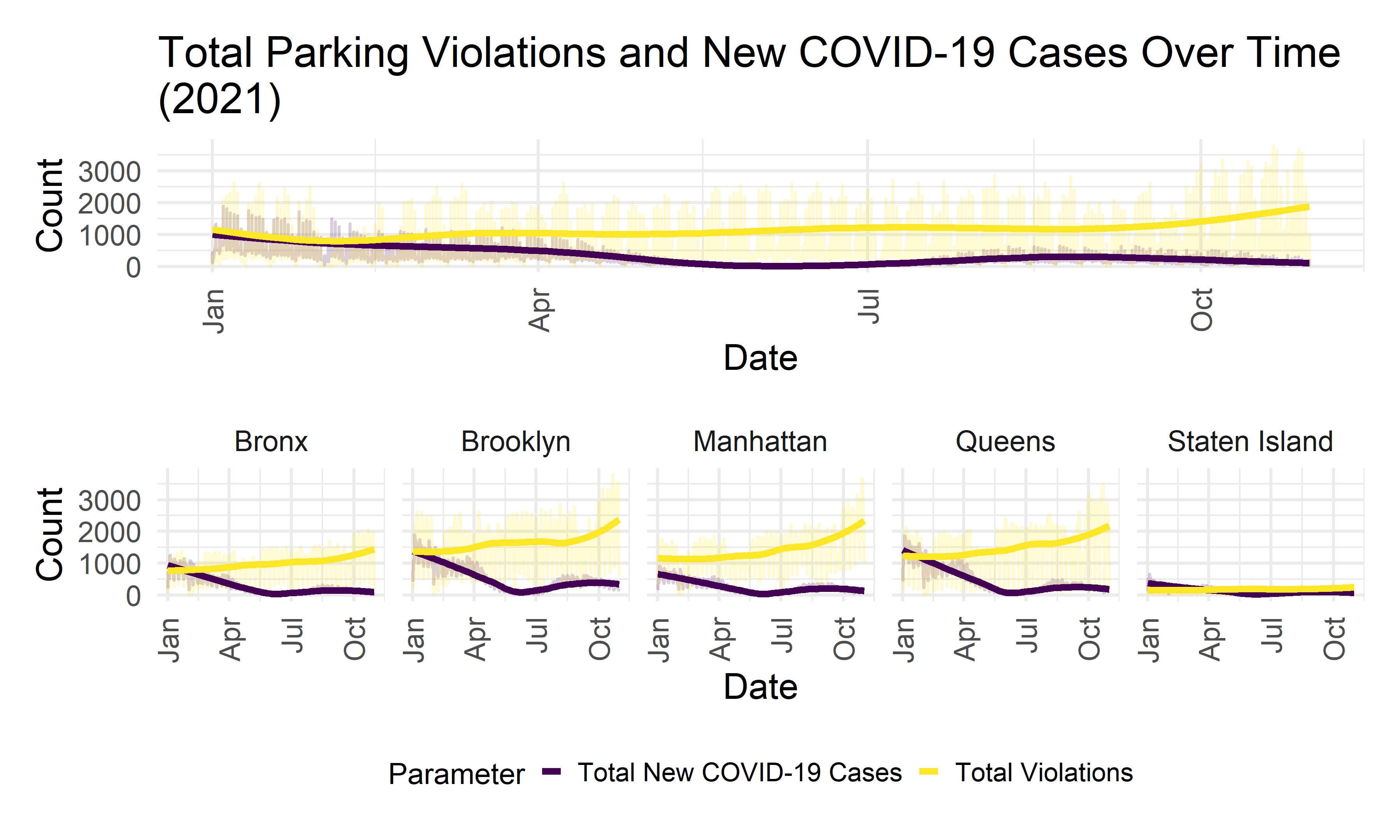

We will now perform a Granger-causality test to see if knowing the previous day’s number of COVID-19 cases is helpful in predicting the number of parking violations given out. We will perform this test at an $\alpha = 0.05$ significance level.

grangertest(total_violations ~ new_cases, order = 1, data = violation_covid)

## Granger causality test
## 
## Model 1: total_violations ~ Lags(total_violations, 1:1) + Lags(new_cases, 1:1)
## Model 2: total_violations ~ Lags(total_violations, 1:1)
##   Res.Df Df      F    Pr(>F)    
## 1   1516                        
## 2   1517 -1 47.147 9.575e-12 ***
## ---
## Signif. codes:  0 '***' 0.001 '**' 0.01 '*' 0.05 '.' 0.1 ' ' 1

As the test’s p-value is less than our predetermined significance level of 0.05, we reject the null hypothesis that a model only based on the total violations time series performs as well or out performs a model that is based on both the total violations time series and COVID-19 case count time series. Thus, there is at least some predictive causality between the daily count of COVID-19 cases and the total daily parking violations over the past year.

Is the distribution of violation types different across boroughs?

We are also interested in knowing whether there is difference in the counts of ticket amounts in the city-wide top 5 violation types in different boroughs. To do this, we perform a chi-squared test to test the homogeneity of violation types across boroughs in the top 5 violation types overall.

Chi-square Test - Top 5 Violation Types and Boroughs

$H_0:$ the expected counts in each violation type category are the same across all boroughs.

$H_1:$ the expected counts in each violation type category are not same across all boroughs.

## 1) No parking-street cleaning, 2) Failure to display a muni-meter receipt, 3) Inspection sticker-expired/missing, 4) Registration sticker-expired /missing, and 5) Fire hydrant. 

five_common_violation = 
  violation1 %>%
  select(borough, violation) %>% 
  filter(violation %in%
           c("NO PARKING-STREET CLEANING",
             "FAIL TO DSPLY MUNI METER RECPT",
             "INSP. STICKER-EXPIRED/MISSING",
             "REG. STICKER-EXPIRED/MISSING",
             "FIRE HYDRANT")) %>%
  count(violation, borough) %>% 
  pivot_wider(
    names_from = "violation",
    values_from = "n"
  ) %>% 
  data.matrix() %>% 
  subset(select = -c(borough))

rownames(five_common_violation) <- c("Bronx", "Brooklyn", "Manhattan", "Queens", "Staten Island")

five_common_violation %>% 
  knitr::kable(caption = "Results Table")

Results Table
	FAIL TO DSPLY MUNI METER RECPT	FIRE HYDRANT	INSP. STICKER-EXPIRED/MISSING	NO PARKING-STREET CLEANING	REG. STICKER-EXPIRED/MISSING
Bronx	24005	32407	44436	46874	35410
Brooklyn	49347	43903	67654	101494	51038
Manhattan	49902	31794	40856	43963	35280
Queens	72767	31610	61256	60778	56589
Staten Island	6025	1946	15857	16	13492

chisq.test(five_common_violation)

## 
##  Pearson's Chi-squared test
## 
## data:  five_common_violation
## X-squared = 53839, df = 16, p-value < 2.2e-16

x_crit = qchisq(0.95, 16)
x_crit

## [1] 26.29623

The result of chi-square shows that $\chi^2 > \chi_{crit}$, at significant level $\alpha = 0.05$, so our result is statistically significant and we can conclude that there does exist at least one borough’s proportion of violation amounts in the top 5 violation types is different from others.

Did equal proportions of the population in each borough receive fire hydrant parking violations in the past year?

Now, we want to see whether receiving a fire hydrant violation is am equally common occurrence within the residents of each borough. To do this, we will conduct a proportion test.

Proportion Test

Since the population vary from boroughs, we want to standardize the population to assure the accuracy of former test results. We first derived the population of each borough from the most recent census. Next, we performed a proportion test to examine whether the proportion of fire hydrant violations (against the total population in each borough) differs across boroughs.

We will also assume:

Each car has only one driver;
Each car gets one fire hydrant violation in 2021.

$H_0:$ The proportion of the individuals who experienced getting a fire hydrant is the same across all boroughs.

$H_1:$ The proportion of the individuals who experienced getting a fire hydrant is not the same across all boroughs.

url = "https://www.citypopulation.de/en/usa/newyorkcity/"
nyc_population_html = read_html(url)

population = nyc_population_html %>% 
  html_elements(".rname .prio1") %>% 
  html_text()

boro = nyc_population_html %>% 
  html_elements(".rname a span") %>% 
  html_text()

nyc_population = tibble(
  borough = boro,
  population = population %>% str_remove_all(",") %>% as.numeric()
) 
  
fire_hydrant = violation1 %>%
  select(borough, violation, plate) %>% 
  filter(violation == "FIRE HYDRANT") %>%
  distinct(plate, borough) %>% 
  count(borough) 

boro_population = left_join(fire_hydrant, nyc_population)

boro_population %>% 
  knitr::kable(caption = "Results Table")

Results Table
borough	n	population
Bronx	18432	1472654
Brooklyn	28124	2736074
Manhattan	20809	1694251
Queens	21832	2405464
Staten Island	1611	495747

prop.test(boro_population$n, boro_population$population)

## 
##  5-sample test for equality of proportions without continuity
##  correction
## 
## data:  boro_population$n out of boro_population$population
## X-squared = 4127.7, df = 4, p-value < 2.2e-16
## alternative hypothesis: two.sided
## sample estimates:
##      prop 1      prop 2      prop 3      prop 4      prop 5 
## 0.012516178 0.010278962 0.012282123 0.009076004 0.003249641

From the above results, p-values are small and so we we can say that the proportions of people getting fire hydrant violations are different across boroughs.

Mapping and Spatial Analysis

Finally, we would like to create some maps of fire hydrant violations by borough. We also want to investigate whether we can find hydrants that are most frequently ticketed.

Geolocation (NYCGeoSearch)

After trying several different geolocating methods, we found that NYCGeoSearch provides the best platform to obtain geographical coordinates (latitude, longitude) from the street addresses we were provided. This platform is advantageous as we can manipulate the search terms by altering the website’s URL. After passing the website into the fromJSON() function from the jsonlite package, we can scrape the page for the data we are interested in (coordinates and borough).

hydrant <- 
  violation %>% 
  filter(violation %in% c("FIRE HYDRANT"), !is.na(geo_nyc_address)) 

pb <- progress_bar$new(total = nrow(hydrant)) # adding progress bar for sanity

get_coord <- function(url) {
  pb$tick()
  
  json_output <- fromJSON(url(url))$features
  
  coord <- json_output$geometry[2]
  borough <-  json_output$properties$borough
  
  out_df <- 
    tibble(
      coordinates = coord$coord,
      mapped_borough = borough
    )
  return(out_df)
}

hydrant_lat_long <- 
  hydrant %>%
  mutate(
  new_url = paste0("https://geosearch.planninglabs.nyc/v1/search?text=", geo_nyc_address, "&size=25"),
  coord = map(new_url, get_coord)
) %>%
  unnest(coord) %>%
  filter(mapped_borough == borough)

The address information provided in our raw data is not very complete and not standardized, as some observations are missing address components (such as house number or street name) and some observations have address components that are not recognizable by the platform (i.e. “30 feet west of Broadway”). As such, the platform produces many possible coordinates for some addresses while not being able to find any coordinates for other observations.

We will work with only the observations that NYCGeoSearch was able to find location coordinates for. We will further restrict this dataset to only include coordinate results that were in the same borough as reported on the citation, and then select just the first coordinate results, if multiple exist.

Finally, we will process the resulting list column through a for loop to extract the latitude and longitudes from each coordinate to their own columns (named lat and long).

hydrant_lat_long <-
  hydrant_lat_long %>%
  group_by(summons_number, geo_nyc_address) %>%
  slice(1)

for (i in 1:nrow(hydrant_lat_long)) {
  hydrant_lat_long$lat[i] <- hydrant_lat_long$coordinates[[i]][2]
  hydrant_lat_long$long[i] <- hydrant_lat_long$coordinates[[i]][1]
}

Running through all previous code chunks up until here takes approximately 7 hours. We will go ahead and save the output from running this code in hydrant_lat_long.csv so that we can read the data from this file into R, instead of running the previous chunks.

write_csv(hydrant_lat_long, "data/hydrant_lat_long.csv")

We will also load a dataset containing locations of all fire hydrants in NYC, from a file named Hydrants.csv. After tidying and recoding some of the variables, we end up with a dataset where each record corresponds with a single fire hydrant. This dataset will contain the variables borough (borough the fire hydrant is located in), unitid (hydrant identifier), and lat and long (hydrant lat/long coordinates).

hydrant_lat_long <- read_csv("data/hydrant_lat_long.csv") %>% select(-coordinates)

hydrant_lat_long <- hydrant_lat_long %>% mutate(textlab = paste0("Summons Number: ", summons_number, "\nFine Amount: $", fine_amount))

hydrant_actual <- read_csv("data/Hydrants.csv")

hydrant_actual <- 
  hydrant_actual %>%
  mutate(borough = case_when(
    BORO == 1 ~ "Manhattan",
    BORO == 2 ~ "Bronx",
    BORO == 3 ~ "Brooklyn",
    BORO == 4 ~ "Queens",
    BORO == 5 ~ "Staten Island"
  )) %>%
  rename(
    lat = LATITUDE,
    long = LONGITUDE,
    unitid = UNITID
  )

Mapping of Fire Hydrant Violation Locations and Fire Hydrants

We will now plot all the points that we have produced to get a sense of how the fire hydrants are distributed across NYC and where fire hydrant violations occurred in the city.

hydrant_violation_plot <- 
  hydrant_lat_long %>% 
  plot_ly(
    lat = ~lat, 
    lon = ~long, 
    type = "scattermapbox", 
    mode = "markers", 
    alpha = 0.2,
    color = ~borough) %>% 
  layout(
    mapbox = list(
      style = 'carto-positron',
      zoom = 9,
      center = list(lon = -73.9, lat = 40.7)))

hydrant_violation_location_plot <- 
  hydrant_violation_plot %>% 
  add_trace(
  data = hydrant_actual %>% mutate(borough = "Fire Hydrant"),
  lat = ~lat,
  lon = ~long,
  type = "scattermapbox",
  mode = "markers",
  alpha = 0.02,
  color = ~borough
  ) %>% 
  layout(
    mapbox = list(
      style = 'carto-positron',
      zoom = 9,
      center = list(lon = -73.9, lat = 40.7)),
    title = "<b> Parking Violation and Hydrant Location </b>",
     legend = list(title = list(text = "Borough of Violation or Hydrant", size = 9),
                    orientation = "h",
                   font = list(size = 9)))

hydrant_violation_location_plot

This map produces points as expected. We see there are more fire hydrant violations in higher-density areas, particularly regions closer to (or in) Manhattan. We see a similar pattern in the distribution of fire hydrants throughout NYC. If we look a little closer at Manhattan, we can observe some distinct regions of higher fire hydrant violations throughout the borough – notably, around SoHo/downtown, Midtown, around the perimeter of Central Park, and around the Upper East Side.

Commonly Ticketed Fire Hydrants

Finally, we want to find the hydrants that are most commonly ticketed.

According to NYC regulations, cars (or, drivers) are ticketed if they park within 15 feet of a hydrant. We will try to associate violation location points with the fire hydrant that caused the violation by constructing hitboxes of approximately 15 feet in radius around each hydrant and see how many violation points are within those boxes. We will double this radius to somewhat adjust for a lack of precision in the violation coordinates we have obtained. Towards this end, we will construct square hitboxes around our hydrant points such that each side of the square is 60 feet wide.

We will use the function destPoint() from the package geosphere to calculate this. This function takes a latitude and longitude coordinate, a bearing (measured from North), and a distance in meters. We will use this function to obtain the coordinates of the vertices of a square centered around the position of the fire hydrant, 35 feet (10 meters) in radius (measured from center to edge).

After we have done so, we will utilize a few functions from the sp package. First, we will use SpatialPolygons (and associated function Polygons) to construct the squares around each hydrant. Then, the function over will tell us which violation location points land within the hydrant hitboxes we have created.

# distance in meters
d = 10
 
square_coord <- function(lat, long, dist = 5){
 
 point_init <- destPoint(c(long, lat), b = 0, d = dist)
 point1 <- destPoint(point_init, b = 270, d = dist) %>% as.data.frame()
 point2 <- destPoint(point1, b = 180, d = dist*2) %>% as.data.frame()
 point3 <- destPoint(point2, b = 90, d = dist*2) %>% as.data.frame()
 point4 <- destPoint(point3, b = 0, d = dist*2) %>% as.data.frame()
 
 sq <- bind_rows(point1, point2, point3, point4, point1)
 
 x <- sq %>% pull(lat)
 y <- sq %>% pull(lon)
 
 out_mat <- cbind(x, y)
 
 return(out_mat)
}

to_poly <- function(polymat, id){
 poly <- Polygons(list(Polygon(polymat)), ID = id)
 return(poly)
}

first_step <- hydrant_actual %>%
mutate(
  sq = map2(.x = lat, .y = long, ~square_coord(lat = .x, long = .y, dist = d)),
  polys = map2(sq, unitid, to_poly)
)  %>% 
select(polys) %>%
pull(polys)

squares <- SpatialPolygons(first_step)

# now, get points ready 

x = hydrant_lat_long %>% pull(lat)
y = hydrant_lat_long %>% pull(long)
xy = cbind(x,y)

dimnames(xy)[[1]] = hydrant_lat_long %>% pull(summons_number)
pts = SpatialPoints(xy)
  
# check if drawn squares have points in them
hits <- over(squares, pts, returnList = TRUE)


hit_hydrants <- tibble(id = names(hits), hits = hits)
hit_hydrants1 <- hit_hydrants %>% unnest(hits)
hit_hydrants2 <- hit_hydrants1 %>% group_by(id) %>% summarise(num_hits = n()) %>% arrange(-num_hits)

isolated_hydrants <- inner_join(hydrant_actual, hit_hydrants2, by = c("unitid" = "id"))

We see that there are 837 hydrants. We will first reverse geocode the hydrant coordinates to allow the output to be more useful to the human user. We will use the revgeo function from the revgeo package and use Google’s reverse geocode API to get the addresses. Since using Google’s API is not exactly free, we will perform this once and save the addresses in a CSV file.

hydrant_loc <- revgeo(isolated_hydrants %>% pull(long), isolated_hydrants %>% pull(lat), provider = "google", API = "API") # API key has been removed

address <- hydrant_loc %>% unlist()
hydrant_loc <- bind_cols(isolated_hydrants, address = address)

write_csv(hydrant_loc, "data/isolated_hydrant_loc.csv")

Let’s now create our plot!

isolated_hydrants <- read_csv("data/isolated_hydrant_loc.csv")

isolated_hydrants_plot <- 
  isolated_hydrants %>%
  mutate(
    borough = "Hydrant",
    textlab = paste0("Number of Associated Violations: ", num_hits, "\nAddress: ", address)
    ) 

hydrant_plot <- 
  hydrant_lat_long %>% 
  plot_ly(
    lat = ~lat, 
    lon = ~long, 
    type = "scattermapbox", 
    mode = "markers", 
    alpha = 0.01,
    color = ~borough,
    text = ~textlab,
    colors = "viridis")

plot <- hydrant_plot %>% add_trace(
  data = isolated_hydrants_plot,
  lat = ~lat,
  lon = ~long,
  type = "scattermapbox",
  mode = "markers",
  size = ~num_hits,
  text = ~textlab,
  color = ~borough,
  marker = list(
    color = "red"
    ),
  alpha = 0.5
  )

plot %>% layout(
    mapbox = list(
      style = 'carto-positron',
      zoom = 9,
      center = list(lon = -73.9, lat = 40.7)),
      title = "<b> Most Frequently Ticketed Hydrants</b>",
     legend = list(title = list(text = "Borough of Violation or Hydrant", size = 9),
                    orientation = "h",
                   font = list(size = 9)))

Interestingly, it seems that the hydrant whose hitbox intersected the most violation points is located in Brooklyn. The following table shows the ten most frequently ticketed hydrants:

hydrants_table <- 
  isolated_hydrants %>% 
  arrange(-num_hits) %>% 
  filter(row_number() <= 10) %>%
  select(unitid, address, num_hits) %>%
  rename(
    c("Hydrant ID" = "unitid", "Hydrant Address" = "address", "Number of Tickets" = "num_hits")
  )
  hydrants_table %>% knitr::kable()

Hydrant ID	Hydrant Address	Number of Tickets
H301940	2 Atlantic Ave., Pier 7, Brooklyn, NY 11201, USA	40
H202171	522 Morris Ave, Bronx, NY 10451, USA	34
H311717	150 Graham Ave, Brooklyn, NY 11206, USA	26
H107599	25 James St, New York, NY 10038, USA	21
H420999	197-50A Peck Ave, Fresh Meadows, NY 11365, USA	16
H205952	530 E 144th St, Bronx, NY 10454, USA	15
H203269	1468 College Ave, Bronx, NY 10457, USA	15
H101773	Minetta Green, S/e Corner Minetta Lane and, 6th Ave, New York, NY 10012, USA	14
H332046	8 Old Fulton St, Brooklyn, NY 11201, USA	14
H326869	11 Schenck Ct, Brooklyn, NY 11207, USA	13

It is important to note that the above spatial analysis will only be as precise as the geocoded violation coordinates will be.

Next Steps and Discussion

At first, we were interested in seeing if any conclusions can be made about the frequency at which specific parking violations are given out and if there are any factors that may be associated to receiving one in 2021, as stated in the proposal. Therefore we investigated the boroughs that had the most violations, the borough paid the most in fines and other general topics.

After we began, we narrowed down the range of the topic focus. We did research on the distribution of violations in other variables such as the dataset borough, date, vehicle type, nearby fire hydrants. The most curious factor was the fire hydrants. Were the number of parking violations related to fire hydrants the same across the five boroughs? Following the question, we decided to find the hydrants that seem to be ticketed the most commonly.

To start with, we wanted to build the mapping for the distribution of parking violation spots. We exported the complete parking violation address from the Parking Violations Issued - Fiscal Year 2021 dataset. The package of tidygeocoder made getting data from geocoding services easy. We imported the address data and get the return of latitudes and longitudes via Google Api. Dropping the null value, we obtained the csv file containing latitudes and longitudes of parking violation address. Then we adopted the file to visualize geographical data on the map in kepler. The shining points revealed the parking violation sites distribution.

However, the speed of data analysis severely depended on WIFI speed because we relied on the Google API to get the file containing latitudes and longitudes for parking violation address. So we dropped the thought and searched for more practical methods.

Soon, we found that NYCGeoSearch provides the best platform to obtain geographical coordinates (latitude, longitude) from the street addresses we were provided. This platform is advantageous as we can manipulate the search terms by altering the website’s URL. After passing the website into the fromJSON() function from the jsonlite package, we can scrape the page for the data we are interested in (coordinates and borough). Then we painted the graphic of the distribution of suspicious hydrants that may cause the violation tickets and performed the mapping and data analysis.

Findings and Summary

Brooklyn has the highest number of tickets among five boroughs. Manhattan and Queens have approximately the same number of tickets.
There is a sharp increase in number of tickets in October in all boroughs.
Top three types of violation: No Parking-Street Cleaning, Inspection Sticker Expired/Missing, Fail to Display a muni-meter receipt.
Saturday has the lowest violation counts and Friday had the second lowest counts comparing to all other weekdays.
Violation increases from 6:00 AM to 8:00 AM, remains high in 8:00 AM to 2:00 PM, decrease from 2:00 PM to 7:00 PM.
Average fine amount is highest in Manhattan and lowest in Staten Island. There is significant difference between fine amounts and at least 2 boroughs.
Suburban(SUBN) is the vehicle type that has the highest number of violation.

Statistical Analysis Findings:

ANOVA test: the parking violation counts are associated with month and weekday.
Chi-square test: the proportions of violation amounts is different among boroughs.
Proportion test: the proportions of people getting fire hydrant violations are different across boroughs.

Limitations and Reflections

There are also several limitations for our project. The major challenge would be the data cleaning process, especially for our first dataset - Open Parking and Camera Violations. As the dataset is too large to download and run in R, we only focused in 2021. Also, there are some future observations after the date we downloaded the dataset which should not be there, so we just excluded these observations in the data cleaning process. We noticed that this dataset is keeping updated every few months, if we want to explore more of this dataset, maybe we can keep tracking for the update and download it right after it’s last update, then check if the dataset’s date is consistent with the data update date.

Additionally, the maps we have produced are limited by the quality of street location data we have been provided. Though it would be best for the data quality itself to improve, if a more precise map is desired and resources are available, we would recommend using a more sophisticated API to geocode street locations to coordinates.

Influence - Feasible Application

Our project can make an impact on the community. To be more specific, if merging our findings of fire hydrants locations in NYC to a commonly used geolocating system (such as GoogleMaps), and generating an alert when parking within the safe range (15 feet) of fire hydrants. It could benefit the drivers to follow the parking regulation and avoid getting fire hydrant violations tickets.

A Fun fact – The Poorest Guy

During our analysis process of fire hydrant violation, we found out a license plate JRA7539 got 85 tickets due to fire hydrant in 2021. It’s ridiculous! So we want to find what this car is doing in 2021. The result shows that JRA7539 got a total of 221 violations with fine amount of $19130 this year.

fire_hydrant = violation1 %>% filter(violation == "FIRE HYDRANT")

fire_hydrant_id = violation1 %>% filter(violation == "FIRE HYDRANT") %>% 
  select(issue_date, borough, violation, plate) %>% 
  group_by(plate) %>% 
  filter(n() > 1) %>% 
  distinct(plate) %>% 
  ungroup()
 
 duplicate_hydrant = inner_join(fire_hydrant_id, fire_hydrant, by = "plate")
 
 duplicate_hydrant %>% 
  count(plate) %>% 
   ggplot(aes(x = n)) + 
   geom_histogram()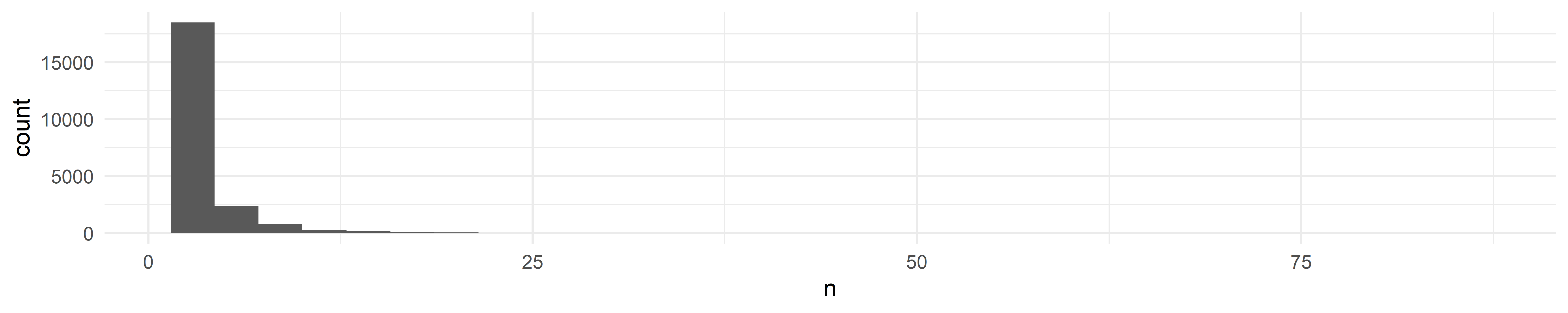

  violation %>% 
     filter(plate == "JRA7539") %>% 
     count(violation) %>% 
     summarize(sum = sum(n))

## # A tibble: 1 x 1
##     sum
##   <int>
## 1   221

   violation %>% 
     filter(plate == "JRA7539") %>% 
     summarize(fine = sum(amount_due))

## # A tibble: 1 x 1
##    fine
##   <dbl>
## 1 19130